
Lecture 1: Jupyter Notebook#
This notebook accompanies Lecture 1. Download it with the button at the top of this page (the .ipynb option), or run it in the browser via the rocket icon once a launch service is configured.
Goals for today
Make sure your Python environment works.
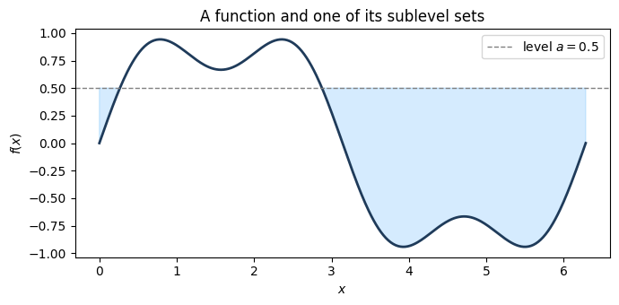
Plot a simple function and locate its critical points.
Math renders inline, e.g. \(f(x) = \sin(x) + \tfrac{1}{3}\sin(3x)\), and in display mode:
\[
f'(x) = \cos(x) + \cos(3x).
\]
import numpy as np
import matplotlib.pyplot as plt

x = np.linspace(0, 2 * np.pi, 400)
f = np.sin(x) + np.sin(3 * x) / 3

fig, ax = plt.subplots(figsize=(7, 3.5))
ax.plot(x, f, lw=2, color="#1f3b5a")
ax.axhline(0.5, ls="--", color="gray", lw=1, label="level $a = 0.5$")
ax.fill_between(x, f, 0.5, where=f <= 0.5, color="#74c0fc", alpha=0.3)
ax.set_xlabel("$x$"); ax.set_ylabel("$f(x)$"); ax.legend(loc="upper right")
ax.set_title("A function and one of its sublevel sets")
plt.tight_layout(); plt.show()
Exercise#
Change the level a in the cell above. For which values of a does the shaded region have one component, and for which does it have two?
# Your code here